


Chapter 28.28
STORM RUNOFF
Sections:
28.28.020 Watershed characteristics.
28.28.030 Time of concentration.
28.28.040 Nonurbanized watersheds.
28.28.050 Urbanized watersheds.
28.28.060 Precipitation losses.
28.28.070 SCS curve number method.
28.28.090 Green and Ampt method.
28.28.100 Rational formula method.
28.28.110 SCS unit hydrograph method.
28.28.120 Channel routing of hydrographs.
28.28.130 Reservoir routing of hydrographs.
28.28.010 Introduction.
For the area within the jurisdiction of this manual, two deterministic hydrological models can be used to estimate storm runoff, rational formula and the SCS unit hydrograph method. The techniques for these methods are presented in this chapter.
The rational and SCS unit hydrograph methods require the user to determine watershed characteristics (i.e., area, length, slope, imperviousness, etc.) and the characteristic response time for the watershed (time of concentration). The SCS unit hydrograph method also requires calculation of the precipitation losses. Procedures for these parameters are presented first, followed by specific requirements for each method.
For certain circumstances, where adequate recorded stream flow data are available and the watershed area is large (greater than 10 square miles), a statistical analysis may be required to predict the storm runoff peaks or for calibration of deterministic models.
(Res. 40-08 (§ 701), 3-19-08)
28.28.020 Watershed characteristics.
The watershed characteristics needed for the runoff computation methods include the watershed area, the various flow path lengths, slopes, and surface conditions (i.e., overland, grassed channel, gutter), soil infiltration rates, and land use or imperviousness.
(a) Physical Features. Watershed boundaries and areas can be determined from topographic maps, but a field investigation is recommended to verify boundaries. Land use and flow path characteristics can be obtained from zoning maps, aerial photographs, field investigations, or detailed topographic maps. Soil characteristics can be determined from NRCS (formerly SCS) soil reports for Mesa County.
(b) Watershed Imperviousness. Imperviousness, Imp, is a basic characteristic that is a direct measure of the watershed’s potential to produce storm runoff in terms of peak rates and total runoff volume. It is also a predictive indicator of watershed response to urbanization and the subsequent impact on stream stabilization and water quality.
Imperviousness is used in the rational method to derive the runoff coefficient and can be used in the SCS unit hydrograph method to derive runoff curve number. Imperviousness is typically determined in one of two ways, either by identification of watershed surface conditions (i.e., natural ground versus hard surfaces) and direct computation or by characterization of the land uses (i.e., undeveloped, residential, commercial, industrial) which have typical values of imperviousness.
Recommended impervious values for surface conditions and for typical land use types are provided in Table 28.28.020. The more precise approach is to divide the watershed into pervious and impervious surfaces and then compute the overall imperviousness directly, which is the required method for determining imperviousness for new development. This approach can be used when aerial photographs or detailed development plans (i.e., for planned unit developments) are available, or field investigations of existing conditions are performed.
When this information is not available or for projecting watershed imperviousness for future land uses, then typical imperviousness values from Table 28.28.020 are used. For single-family residential development when the housing density (i.e., units per acre) and the size and type of housing (i.e., ranch, split level, and two-story) can be determined, then the use of Figures 28.28.020(a), 28.28.020(b) and 28.28.020(c) is recommended. These figures are indicative of the existing development trend to place larger houses, including driveways, walks, patios, and outbuildings, on smaller lots. However, imperviousness values have also been found to be representative of older developments with small lots where additional impervious surfaces were added over time.
Note that in undeveloped areas that are to remain undeveloped, two percent imperviousness may be used for all areas that have soil and vegetative cover. However, these undeveloped areas often have significant geological features such as rock outcroppings that must be accounted for by calculating a composite imperviousness for these basins. Rock outcroppings are typically assigned an imperviousness of 100 percent for these calculations.

Figure 28.28.020(a): Watershed Imperviousness, Single-Family Residential Ranch Style House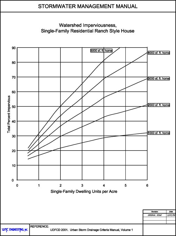
Figure 28.28.020(b): Watershed Imperviousness, Single-Family Residential Split Level House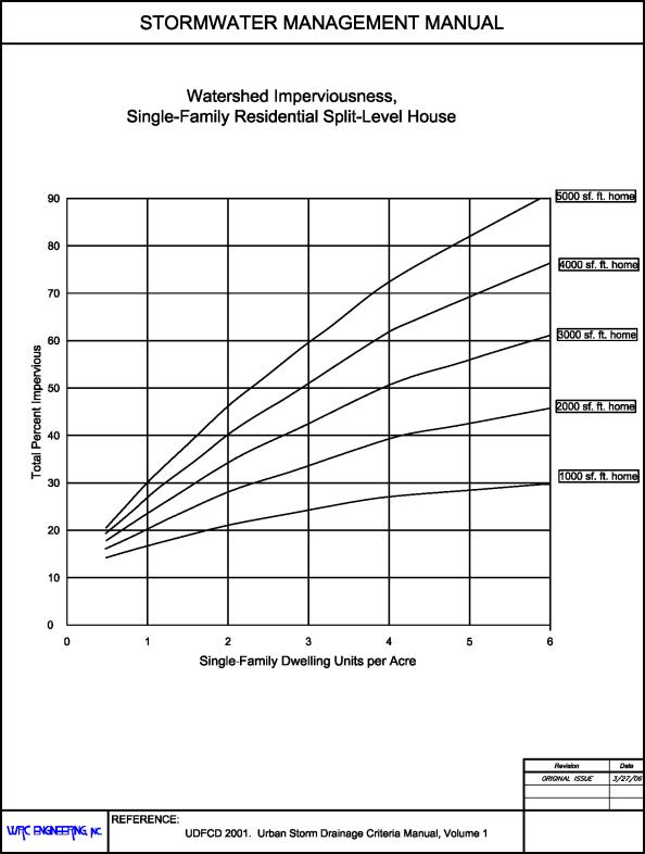
Figure 28.28.020(c): Watershed Imperviousness, Single-Family Residential Two-Story House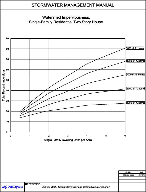
(Res. 40-08 (§ 702), 3-19-08)
28.28.030 Time of concentration.
The time of concentration, tc, is the time required for runoff to flow from the most remote part of the watershed area to the point of interest. For the rational formula, the time of concentration is calculated so that the average rainfall rate for a corresponding duration can be determined from the rainfall intensity-duration-frequency curves. For the SCS unit hydrograph methods, the time of concentration is used to determine the time-to-peak, tp, of the unit hydrograph and subsequently, the peak runoff.
For consistency between runoff analyses, the time of concentration equations presented in this chapter shall be used for all small watershed (less than 1.0 square miles) runoff calculations. For large watershed calculations, the watershed lag equation for the SCS unit hydrograph method is recommended (see GJMC 28.28.110(c)).
Time of concentration consists of an initial time or overland flow time, ti, plus travel time, tt, which is in a combined form. In both urban and nonurban environments, the initial or overland flow is assumed to occur as sheet flow and as a function of surface type and slope, with an upper limit on the distance which this type of flow can occur.
(Res. 40-08 (§ 703), 3-19-08)
28.28.040 Nonurbanized watersheds.
For nonurban areas, the travel time occurs in a combined form, such as a small swale, channel, or wash. In urban areas, the travel time occurs in a combined form, such as in the storm drain, paved gutter, roadside drainage ditch, or drainage channel. Travel time can be estimated from the hydraulic properties of the storm drain, gutter, swale, ditch, or wash. Initial time, on the other hand, will vary with surface slope, depression storage, surface cover, antecedent rainfall, and infiltration capacity of the soil, as well as distance of surface flow.
The time of concentration for both urban and nonurban areas is calculated as follows:
|
tc |
= |
ti + tt |
(28.28-1) |
Where:
|
tc |
= |
Time of concentration (min) |
|
ti |
= |
Initial, inlet, or overland flow time (min) |
|
tt |
= |
Travel time in the ditch, channel, gutter, storm drain, etc. (min) |
Standard Form No. 2 has been developed to organize the calculation of tc.
The initial or overland flow time, ti, may be calculated using the following equation:
|
ti |
= |
1.8 (1.1 – K) Lo1/2 / S1/3 |
(28.28-2) |
Where:
|
ti |
= |
Initial or overland flow time (min) |
|
K |
= |
Flow resistance coefficient |
|
Lo |
= |
Length of overland flow (feet, 300-foot maximum) |
|
S |
= |
Average watershed slope (percent) |
Equation 28.28-2 was originally developed by the Federal Aviation Administration (FAA, 1970) for use with the rational formula method. However, the equation is also valid for computation of the initial or overland flow time for the SCS unit hydrograph method. The five-year runoff coefficient, C5, presented in Table 28.28.040(a) is recommended for the flow resistance coefficient, K.
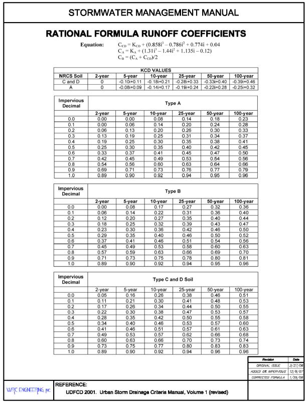
Figure 28.28.040: Travel Velocity for Rational Method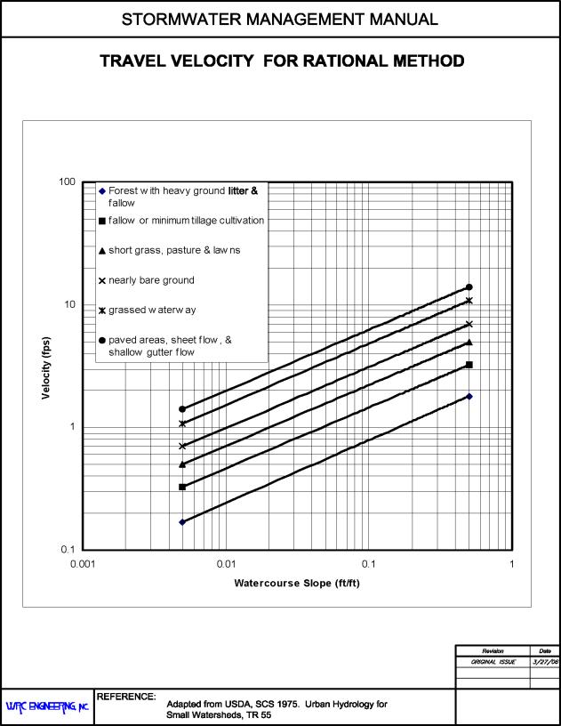
The overland flow length, Lo, is generally defined as the length over which the flow characteristics appear as sheet flow or very shallow flow in broad, grassed swales. Changes in land slope, surface characteristics, and small drainage ditches or gullies will tend to force the overland flow into a combined flow condition, which results in higher flow velocities and shorter travel times. Therefore, the initial flow time is limited to the time to travel a distance of 300 feet.
For watersheds longer than 300 feet, the travel time, tt, must be added to the overland flow time. Travel time can be calculated using Manning’s equation and the hydraulic properties of the storm drain, gutter, swale, ditch, or channel or can be approximated from Equation 28.28-3 and Figure 28.28.040:
|
V |
= |
Cv Sw0.5 |
(28.28-3) |
Where:
|
V |
= |
Velocity, fps |
|
Sw |
= |
Watercourse slope, ft./ft. |
|
Cv |
= |
Conveyance coefficient |
|
Land Surface |
Conveyance Coefficient Cv |
|---|---|
|
Heavy meadow |
2.5 |
|
Tillage/field |
5.0 |
|
Short pasture and lawns |
7.0 |
|
Nearly bare ground |
10 |
|
Grassed waterways |
15 |
|
Paved areas and shallow swales |
20 |
The time of concentration is then the sum of the initial flow time ti and the travel time tt. The minimum recommended tc for nonurban watersheds is 10 minutes.
(Res. 40-08 (§ 703.1), 3-19-08)
28.28.050 Urbanized watersheds.
Overland flow in urbanized watersheds can occur from the back of the lot to the street, in parking lots, in greenbelt areas, or within park areas and can be calculated using the procedure described in GJMC 28.28.030. Travel time, tt, to the first design point or inlet is often determined based on the conveyance coefficient for paved areas and shallow swales, but can be estimated using Manning’s equation.
The time of concentration for the first design point in an urbanized watershed using this procedure should not exceed the time of concentration calculated using Equation 28.28-4, which was developed using rainfall/runoff data collected in urbanized regions (USDCM, 1969).
|
tc |
= |
L / 180 + 10 |
(28.28-4) |
Where:
|
tc |
= |
Time of concentration at the first design point (min.) |
|
L |
= |
Watershed length (ft.) |
Equation 28.28-4 may result in a lesser time of concentration at the first design point and thus would govern in an urbanized watershed. The recommended minimum tc to the first urban design point is five minutes. For subsequent design points, the time of concentration is calculated by accumulating the travel times in downstream reaches.
(Res. 40-08 (§ 703.2), 3-19-08)
28.28.060 Precipitation losses.
Two methods for calculating precipitation losses are presented below, the SCS curve number and the Green-Ampt methods, both of which can be used for the SCS unit hydrograph method.
Land surface interception, depression storage and infiltration are referred to as precipitation losses. Interception and depression storage represent the surface storage of water by trees or grass, in local depressions in the ground surface, in cracks and crevices in parking lots or roofs, or in a surface area where water is not free to move as overland flow. Infiltration represents the movement of water through the soil beneath the land surface.
Three important factors should be noted about precipitation loss computations. First, precipitation which does not contribute to the runoff process is considered to be lost from the system. Second, the equations used to compute the losses do not provide for soil moisture or surface storage recovery (i.e., contribute to surface runoff); therefore, the calculated amount of runoff is conservatively high. Finally, precipitation losses are considered to be uniformly distributed over an entire sub-watershed.
(Res. 40-08 (§ 704), 3-19-08)
28.28.070 SCS curve number method.
The National Resources Conservation Service (NRCS, formerly SCS), U.S. Department of Agriculture, has instituted a soil classification system for use in soil survey maps across the country. Based on experimentation and experience, the agency has been able to relate the watershed characteristics of soil groups to a curve number, CN (SCS, 1985). The NRCS provides information relating soil group type to the curve number as a function of soil cover, land use type and antecedent moisture conditions, which can be determined from the soil name.
Precipitation loss is calculated based on supplied values of CN and IA, which are related to a total runoff depth for a storm by the following relationships:
|
Q |
= |
(P – IA)2 / ((P – IA) + S) |
(28.28-5) |
|
S |
= |
(1,000 / CN) – 10 |
(28.28-6) |
|
IA |
= |
0.2 S |
(28.28-7) |
Where:
|
Q |
= |
Accumulated excess (in.) |
|
P |
= |
Accumulated rainfall depth (in.) |
|
IA |
= |
Initial abstraction (in.) |
|
S |
= |
Currently available soil moisture storage deficit (in.) |
|
CN |
= |
SCS curve number |
Note that initial abstraction, IA, (i.e., soil surface storage capacity) is based on empirical evidence established by the NRCS, and is the default value in HEC-1 Program (HEC, 1988).
Since the SCS method results in total excess for a storm, the incremental excess (the difference between rainfall and precipitation loss) for a time period is computed as the difference between the accumulated excess at the end of the current period and the accumulated excess at the end of the previous period.
(Res. 40-08 (§ 704.1), 3-19-08)
28.28.080 CN determination.
The SCS curve number method uses a soil cover curve number (CN) for computing excess precipitation. The curve number CN is related to hydrologic soil group (A, B, C, or D), land use, treatment class (cover), and antecedent moisture condition.
The soil group is determined from published soil maps for the area, which correlates each soil name with the soil group. Land use and treatment class are determined during field visits or from aerial photographs. Procedures for determining land use and treatment class are found in Chapter 8 of National Engineering Handbook, Section 4 (SCS, 1985). Antecedent moisture condition of the watershed is explained as follows:
The amount of rainfall in a period of five to 30 days preceding a particular storm is referred to as antecedent rainfall, and the resulting condition of the watershed in regard to potential runoff is referred to as an antecedent moisture condition. In general, higher amounts of antecedent rainfall result in greater amounts of runoff from a given storm. The effects of infiltration and evapotranspiration during the antecedent period are also important, as they may increase or lessen the effect of antecedent rainfall. Because of the difficulties of determining antecedent storm conditions from data normally available, the conditions are reduced to three cases, AMC-I, AMC-II and AMC-III. For the Mesa County area, an AMC-II condition is recommended for determining storm runoff.
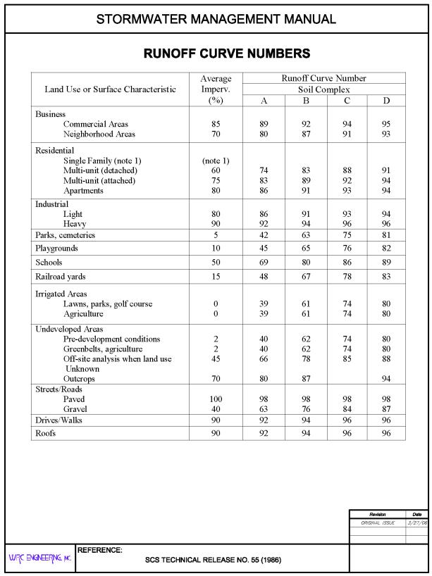
Having determined the soil group, land use and treatment class and the antecedent moisture condition, CN values can be determined from Table 28.28.080, which is reproduced from Table 2-2 in TR-55 (SCS, 1986).
When land uses shown in Table 28.28.080 are not applicable or when more detailed land use information is available, CN values can be calculated directly from imperviousness estimates using the following equation.
|
CN |
= |
98*Imp + X*(1-Imp) |
(28.28-8) |
Where:
|
Imp |
= |
Imperviousness as a decimal |
|
X |
= |
Adjustment factor based on NRCS Soil Type |
|
NRCS Soil Type |
Adjustment Factor |
|---|---|
|
A |
39 |
|
B |
61 |
|
C |
74 |
|
D |
80 |
Note that Equation 28.28-8 was derived from the data plotted on Figure 2-3 in TR-55 (SCS 1986) and applies when impervious surfaces are connected. Adjustment for disconnected impervious surfaces can be made using Figure 2-4 in TR-55. This adjustment is not required as the connected impervious surface assumption will result in conservatively high CN values.
(Res. 40-08 (§ 704.2), 3-19-08)
28.28.090 Green and Ampt method.
The Green-Ampt method models infiltration by combining an unsaturated flow form of Darcy’s law with requirements of mass conservation. The Green-Ampt method involves the simulation of rainfall loss as a two-phase process. The first phase of rainfall loss is called initial abstraction (IA) or surface retention loss, which involves vegetation interception, evaporation, and surface depression storage. Typical surface retention loss values are shown in Table 28.28.090(a).
|
Land Use and/or Surface Cover |
Surface Retention Loss, IA (inches) |
|---|---|
|
Natural |
|
|
Desert and rangeland, flat slope |
0.35 |
|
Desert hillslopes |
0.15 |
|
Mountain with vegetated surface |
0.25 |
|
Developed (residential/commercial) |
|
|
Lawn and turf |
0.20 |
|
Desert landscape |
0.10 |
|
Pavement |
0.05 |
|
Agricultural, tilled fields and irrigated pasture |
0.50 |
The second phase of the rainfall loss process is infiltration of rainfall into the soil. The infiltration is assumed to begin after the surface retention loss is completely satisfied. Excess precipitation is computed using the Green-Ampt equations after the initial loss is satisfied. Required parameters are then the hydraulic conductivity of the soil at saturation, volumetric moisture deficit at the beginning of rainfall, and wetting front capillary action.
Typical values for Green-Ampt parameters were obtained from the Drainage Design Manual for Maricopa County Hydrology (Maricopa County 2003 (draft)), available at:
http://www.fcd.maricopa.gov/Resources/HydrologyManual.asp.
(a) Soil Hydraulic Conductivity. The soil hydraulic conductivity is based on soil texture classification. Typical values for different soil type are listed in Table 28.28.090(b). For watershed areas of sub-watersheds consisting of several different soil textures, a composite value for Green-Ampt parameters should be used.
|
Soil Texture Classification |
Hydrologic Soils Group |
Soil Hydraulic Conductivity (in/hr) |
|---|---|---|
|
Loamy-sand and sand |
A |
1.20 |
|
Sandy-loam |
B |
0.40 |
|
Loam |
B |
0.25 |
|
Silty-loam |
C |
0.15 |
|
Sandy clay-loam |
C |
0.06 |
|
Clay-loam |
D |
0.04 |
|
Silty clay-loam |
D |
0.04 |
|
Sandy-clay |
D |
0.02 |
|
Silty-clay |
D |
0.02 |
|
Clay |
D |
0.01 |
Hydraulic conductivity is affected by several factors besides soil texture, including soil crusting, tillage, ground cover, and canopy cover and should be adjusted. Ground cover, such as grass, litter, and gravel, will generally increase the infiltration rate over that of bare ground conditions. Canopy cover, such as from trees, brush, and tall grasses, also increases the bare ground infiltration rate. A simplified procedure for adjusting bare ground hydraulic conductivity to account for vegetation cover is provided in Equation 28.28-9:
|
Ck |
= |
(Vc-10)/90 + 1.0 |
(28.28-9) |
Where:
|
Ck |
= |
Hydraulic conductivity ratio to bare ground conductivity |
|
Vc |
= |
Vegetated cover as a percentage |
(b) Volumetric Soil Moisture Deficit. The soil moisture deficit is a volumetric measure of the soil moisture-storage capacity that is available at the start of the rainfall. The volumetric moisture deficit is a function of the effective porosity of the soil and its value is in the range of near zero to the effective porosity. If the soil is saturated at the start of rainfall, then the moisture deficit equals zero. If the soil is devoid of moisture at the start of rainfall, then the moisture deficit is essentially the effective porosity of the soil.
Three conditions for soil moisture deficit have been defined for use based on the antecedent soil moisture condition that could be expected to exist at the start of the design rainfall. These three conditions are:
(1) “Dry” for antecedent soil moisture near the vegetation wilting point;
(2) “Normal” for antecedent soil moisture condition near field capacity due to previous precipitation or land irrigation; and
(3) “Saturated” for antecedent soil moisture near effective saturation due to recent precipitation or land irrigation.
Typical volumetric soil moisture deficit values for the above three defined conditions may be taken from Figure 28.28.090. For Mesa County, the recommended condition is “normal,” which is consistent with antecedent moisture condition II.
(c) Wetting Front Capillary Action. This parameter is relatively insensitive to ground cover, and is a function of the average bare soil type hydraulic conductivity. Typical values may be taken from Figure 28.28.090.
Figure 28.28.090: Adjustment for Soil Moisture Deficit and Capillary Action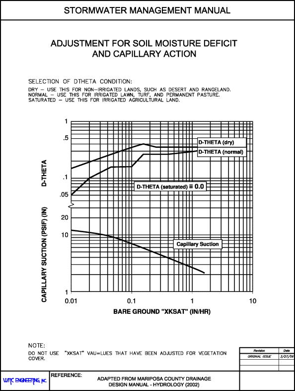
(Res. 40-08 (§ 704.3), 3-19-08)
28.28.100 Rational formula method.
For watersheds that are not complex and have small watershed areas, the design storm runoff may be analyzed using the rational formula method. This method is widely used due to its simplicity and level of general acceptance. The rational formula method, when properly applied in a consistent manner, results in drainage facilities sizes that adequately convey storm runoff with minimal consequences.
(a) Methodology. The rational method is based on the formula:
|
Q |
= |
CIA |
(28.28-10) |
Where:
|
Q |
= |
Maximum rate of runoff in cubic feet per second (cfs) |
|
C |
= |
Runoff coefficient |
|
I |
= |
Average intensity of rainfall in inches per hour |
|
A |
= |
Contributing watershed area in acres |
(b) Assumptions. The basic assumptions made when applying the rational formula method are as follows:
(1) The computed maximum rate of runoff to the design point is a function of the average rainfall rate during the time of concentration to that point.
(2) The maximum rate of rainfall occurs during the time of concentration, and the design rainfall depth during the time of concentration is converted to the average rainfall intensity for the time of concentration.
(3) The maximum runoff rate occurs when the entire area is contributing flow.
(c) Limitations on Methodology. The rational formula method adequately estimates the peak rate of runoff from a rainstorm in a given watershed, but does not provide information on the full hydrograph and only approximates the runoff volume.
Typical design procedures assume that all of the design flow is collected at the design point and that there is no carry-over water running overland to the next design point. The problem becomes one of routing the surface and subsurface hydrographs which have been separated by the storm drain system. In general, this sophistication is not warranted and a conservative assumption is made that the entire routing occurs through the storm drain system when the system is present.
Because of the limitations of the rational method, the following guidelines on its application are provided:
(1) The individual sub-watershed sizes should not be greater than 20 acres.
(2) The aggregate of all sub-watershed areas should not be greater than 160 acres.
(3) The sub-watersheds should be reasonably homogeneous for existing and for projected land use.
(d) Rainfall Intensity. The rainfall intensity, I, is the average rainfall rate in inches per hour for the period of maximum rainfall of a given frequency having a duration equal to the time of concentration. Development of rainfall intensities for the rational method is described in Chapter 28.24 GJMC.
(e) Runoff Coefficient. The runoff coefficient, C, represents the integrated effects of infiltration, evaporation, retention, flow routing, and interception, all of which affect the time distribution and peak rate of runoff. Determination of the coefficient requires judgment and understanding on the part of the engineer.
The first step is to determine the composite imperviousness of the watershed using recommended values in Table 28.28.020. Once the imperviousness is determined, recommended C values for various recurrence interval storms are determined from Table 28.28.090 or can be calculated using the following equations:
|
CCD |
= |
KCD + (0.858*i3 – 0.786*i2 + 0.774*i +0.04) |
(28.28-11) |
|
CA |
= |
KA + (1.31*i3 – 1.44*i2 +1.135*i – 0.12) |
(28.28-12) |
|
CB |
= |
(CA + CCD)/2 |
(28.28-13) |
Where:
|
CCD |
= |
Runoff coefficient for C and D soils* |
|
CA |
= |
Runoff coefficient for A soils* |
|
CB |
= |
Runoff coefficient for B soils* |
|
i |
= |
Imperviousness as a decimal |
|
KCD |
= |
Coefficient adjustment for C and D soils |
|
KA |
= |
Coefficient adjustment for A soils |
*If C is not greater than or equal to zero, it should be set to zero.
|
NRCS Soil |
2-year |
5-year |
10-year |
25-year |
50-year |
100-year |
|---|---|---|---|---|---|---|
|
C and D |
0 |
-0.10i+0.11 |
-0.18i+0.21 |
-0.28i+0.33 |
-0.33i+0.40 |
-0.39i+0.46 |
|
A |
0 |
-0.08i+0.09 |
-0.14i+0.17 |
-0.19i+0.24 |
-0.22i+0.28 |
-0.25i+0.32 |
Composite imperviousness is computed on the basis of the percentage of different types of surfaces or land uses in the watershed area. This procedure is often applied to typical sample blocks as a guide to selection of reasonable values of the coefficient for an entire area.
The equations for runoff coefficients as a function of imperviousness and recurrence interval were obtained from the Urban Storm Drainage Criteria Manual by the Urban Drainage and Flood Control District (UDFCD 2001), which can be obtained in .pdf format on the following website:
http://www.udfcd.org/
(f) Application of the Rational Formula Method. The first step in applying the rational formula method is to obtain a topographic map and define the boundaries of all the relevant watersheds. Watersheds to be defined include all watersheds tributary (i.e., off-site areas) to the area of study and sub-watersheds in the study area. A field check is recommended and field surveys may be required in some cases. At this stage of planning, the possibility for the diversion of watershed runoff should be identified.
The major storm watershed does not always coincide with the minor storm watershed. This is often the case in urban areas where a low flow will stay within the gutter and follow the lowest grade, but when a large flow occurs, the flow will be sufficiently deep or flowing with a high velocity such that part of the runoff will overflow street crown and flow into a new sub-watershed.
(g) Major Storm Analysis. When analyzing the major runoff occurring on an area that has a storm drain system sized for the minor storm, care must be used when applying the rational formula method. Normal application of the rational formula method assumes that all of the runoff is collected by the storm drain. For the minor storm design, the time of concentration is dependent upon the flow time in the drain. However, during the major storm runoff, the drains will probably be at capacity and could not carry the additional water flowing to the inlets. This additional water then flows overland past the inlets, generally at a lower velocity than the flow in the storm drains.
If a separate time of concentration analysis is made for the pipe flow and surface flow, a time lag between the surface flow peak and the pipe flow peak will occur. This lag, in effect, will allow the pipe to carry a larger portion of the major storm runoff than would be predicted using the minor storm time of concentration. The basis for this increased benefit is that the excess water from one inlet will flow to the next inlet downhill, using the overland route. If that inlet is also at capacity, the water will often continue on until capacity is available in the storm drain. The analysis of this aspect of the interaction between the storm drain system and the major storm runoff is complex. The simplified and conservative approach of using the minor storm time of concentration for all frequency analyses is acceptable for the Mesa County area.
(Res. 40-08 (§ 705), 3-19-08)
28.28.110 SCS unit hydrograph method.
The SCS unit hydrograph was derived from a large number of natural unit hydrographs from watersheds varying widely in size and geographic location.
(a) Methodology. The SCS unit hydrograph method, which uses the unit hydrograph theory as a basis for runoff computations, computes a hydrograph for a unit amount of rainfall excess applied uniformly over a sub-watershed for a given unit of time (or unit duration). The rainfall excess hydrographs are then transformed to a sub-watershed hydrograph by superimposing each excess hydrograph lagged by the unit duration.
The shape of the SCS unit hydrograph is based on studies of various natural unit hydrographs. The basic governing parameters of this curvilinear hydrograph are as follows:
(1) The time-to-peak, Tp, of the unit hydrograph approximately equals 0.2 times the time-of-base, Tb.
(2) The point of inflection of the falling leg of the unit hydrograph approximately equals 1.7 times Tp.
(b) Assumptions. The basic assumptions made when applying the SCS unit hydrograph method (and all other unit hydrograph methods) are as follows:
(1) The effects of all physical characteristics of a given watershed are reflected in the shape of the storm runoff hydrograph for that watershed.
(2) At a given point on a stream, discharge ordinates of different unit graphs of the same unit time of rainfall excess are mutually proportional to respective volumes.
(3) A hydrograph of storm discharge that would result from a series of bursts of excess rain or from continuous excess rain of variable intensity may be constructed from a series of overlapping unit graphs each resulting from a single increment of excess rain of unit duration.
(c) Lag Time. Input data for the SCS dimensionless unit hydrograph method (SCS, 1985) consists of a single parameter, TLAG, which is equal to the lag (in hours) between the center of mass of rainfall excess and the peak of the unit hydrograph.
For small watersheds (less than one square mile) in the Mesa County area, the lag time is related to the time of concentration, tc, by the following empirical relationship:
|
TLAG |
= |
0.6 tc |
(28.28-14) |
Where:
|
TLAG |
= |
The time (hours) between the center of mass of the rainfall excess and the peak of the unit hydrograph. |
|
tc |
= |
The time of concentration (minutes, see GJMC 28.28.030 through 28.28.050). |
For large watersheds (greater than one square mile), the lag time (and tc) is generally governed mostly by the concentrated flow travel time, not the initial overland flow time. In addition, as the watershed gets increasingly larger, the average flow velocity (and associated travel time) becomes more difficult to estimate. Therefore, for these watersheds, the following lag equation is recommended for use in computing TLAG:
|
TLAG |
= |
22.1 Kn (L Lc / S0.5)0.33 |
(28.28-15) |
Where:
|
Kn |
= |
Manning’s roughness factor for the watershed channels |
|
L |
= |
Length of longest watercourse (miles) |
|
Lc |
= |
Watercourse length from the outflow point to a point on the channel nearest the centroid of the watershed (miles) |
|
S |
= |
Average slope of the longest watercourse (feet per mile) |
This lag equation is based on the United States Bureau of Reclamation’s (USBR) analysis of the above parameters for several watersheds in the Southwest desert, Great Basin, and Colorado Plateau area (USBR, 1989). This equation was developed by converting the USBR’s S-graph lag equation to a dimensionless unit hydrograph lag equation.
For watersheds 1.0 square miles in size, it is recommended that the method which results in the shortest TLAG value be used to be conservative.
(d) Roughness Factor. For consistency, recommended roughness factors, Kn, used in the lag time calculation are presented in Table 28.28.110. These factors are based on roughness factor analysis by the USACE (1982) and USBR (1989) as compared to the typical watershed channels found in the Mesa County area. The reader is referred to these documents for further discussion on selection of a proper roughness factor. For multiple land uses within a watershed, composite roughness factors should be determined.
|
Land Use |
Imperviousness % |
Kn |
|---|---|---|
|
Commercial, industrial, office and business |
70 – 85 |
0.05 |
|
Residential |
|
|
|
Rural |
10 – 15 |
0.08 |
|
Low density |
20 – 25 |
0.07 |
|
Medium and high density |
30 – 65 |
0.05 |
|
Irrigated grass, golf courses, parks and cemeteries |
0 – 5 |
0.10 |
|
Undeveloped areas: |
|
|
|
Rock outcroppings |
|
0.04 |
|
Irrigated agriculture |
|
0.10 |
|
Rangelands: |
|
|
|
Grass lands |
|
0.08 |
|
Grass and shrubs |
|
0.09 |
|
Shrub and brush |
|
0.10 |
|
Forest, evergreen |
|
0.15 |
(e) Unit Storm Duration. The minimum unit duration, Δt, is dependent on the time of concentration of a given watershed. As a general rule, the unit storm duration, Δt, should be no greater than Tc/3. For small watersheds (i.e., less than one square mile), the recommended duration is five minutes. For larger watersheds, larger unit durations may be used, but should not exceed 15 minutes.
(f) Sub-Watershed Sizing. The determination of the peak rate of runoff at a given design point is affected by the number of sub-watersheds within a larger watershed. Typically, the more discrete the analysis of a given watershed (more sub-watersheds), the more representative the resulting peak flow is of actual runoff conditions. The improved predictive capability of multiple sub-watersheds is due to better homogeneity of the sub-watershed characteristics, as compared to analysis of the watershed with no sub-watersheds. Recommended guidelines are:
(1) For watersheds up to 100 acres in size, the maximum sub-watershed size should be approximately 20 acres.
(2) For watersheds over 100 acres in size, increasingly larger sub-watersheds may be used as long as the land use and surface characteristics within each sub-watershed are homogeneous. In addition, the sub-watershed sizing should be consistent with the level of detail needed to determine peak flow rates at various design points within a given watershed.
(Res. 40-08 (§ 706), 3-19-08)
28.28.120 Channel routing of hydrographs.
Whenever a large or a nonhomogeneous watershed is being investigated, the watershed should be divided into smaller and more homogeneous sub-watersheds. The storm hydrograph for each sub-watershed is then routed through the channel and combined with individual sub-watershed hydrographs to develop a storm hydrograph for the entire watershed. For hydrograph routing, the Muskingum, kinematic wave, and Muskingum-Cunge methods are recommended for use in the Mesa County area.
The kinematic wave method is recommended when the watershed has well defined channels. The Muskingum-Cunge method is recommended for poorly defined channels that have cross-sections that can be determined from detailed topography or from a cross-section survey, otherwise the Muskingum method is recommended.
(a) Muskingum Method. The Muskingum method estimates some channel storage effects and, as a result, the storm hydrograph shape is modified in translation along a channel reach. The basic equation for the Muskingum method as described by HEC-1 (HEC, 1988) is as follows:
|
|
(28.28-16) |
Where:
|
O2 |
= |
Outflow from the reach at the end of the unit time increment (beginning of the next time increment) |
|
O1 |
= |
Outflow from the reach at the beginning of the time increment |
|
I1 |
= |
Inflow into the reach at the beginning of the time increment |
|
I2 |
= |
Inflow into the reach at the end of the time increment |
|
C1, C2 |
= |
Coefficients defined in Equations 28.28-17 and 28.28-18, respectively |
And
|
C1 |
= |
(2Δt)/[2K(1-X)] + Δt |
(28.28-17) |
|
C2 |
= |
(Δt-2KX)/[2K(1-X)] + Δt |
(28.28-18) |
|
K |
= |
L/(3,600V) |
(28.28-19) |
Where:
|
K |
= |
Muskingum storage time constant in hours |
|
L |
= |
Channel reach length in feet |
|
V |
= |
Translation velocity in fps |
|
Δt |
= |
Unit time increment in hours |
|
X |
= |
Muskingum weighting factor |
The velocity used in Equation 28.28-19 is the wave velocity, which can be estimated for various channel shapes as a function of average velocity, V, for steady uniform flow using Manning’s equation. The approximate wave velocities for different channel shapes are provided below:
|
Channel Shape |
Wave Velocity |
|---|---|
|
Wide rectangular |
5/8 V |
|
Triangular |
4/3 V |
|
Wide parabolic |
11/9 V |
Where V is the velocity from application of the Manning’s equation.
The weighting factor (X) in the Muskingum routing method accounts for the peak flow reduction caused by channel routing. The weighting factor generally varies from 0.0 to 0.5, with 0.0 representing a reservoir type peak reduction and 0.5 representing no peak reduction.
|
Channel Condition |
Weighting Factor “X” |
|---|---|
|
Some storage in over bank but few obstructions (i.e., alluvial fans) |
0.15 |
|
Overbanks with severe obstruction |
0.10 |
The reader is referred to the USBR Flood Hydrology Manual (USBR, 1989) for further discussion on the selection of an appropriate Muskingum weighting factor (X).
The storage constant (K) in the Muskingum routing method accounts for the peak flow translation along a channel reach. This constant is therefore directly related to the reach length and the mean channel flow velocity as shown in Equation 28.28-19. An estimate of the mean channel flow velocity may be obtained using Manning’s formula with the hydraulic radius estimated as being equal to the flow depth. The flow depth (and thus channel flow velocity) is estimated based on the channel cross-sectional shape and the design discharge for the selected flood frequency.
The routing procedure may be repeated for several sub-reaches so the total travel time through the reach is equal to K. To ensure the method’s computational stability and the accuracy of computed hydrograph, the routing reach should be chosen so that:
|
1/[2(1-X)] ≤ K/(ΔT·NSTPS) ≤ 1/(2X) |
(28.28-20) |
Where ΔT is the time increment in hours.
(b) Kinematic Wave Method. In the kinematic wave interpretation of the equations of motion, it is assumed that the bed slope and water surface slope are equal and acceleration effects are negligible.
Thus flow at any point in the channel can be computed from Manning’s formula:
|
Q |
= |
(1.486/n) R2/3 So1/2 A |
(28.28-21) |
Where:
|
Q |
= |
Flow rate, cfs |
|
R |
= |
Hydraulic radius, ft. |
|
So |
= |
Channel bed slope, ft./ft. |
|
A |
= |
Cross-sectional area, square feet |
|
n |
= |
Manning’s resistance factor |
Equation 28.28-21 can be simplified to:
|
Q |
= |
αAm |
(28.28-22) |
Where α and m are related to flow geometry and surface roughness. This is the form of the equation used to route hydrographs through channels.
The kinematic wave method in HEC-1 does not allow for explicit separation of main channel and overbank areas. Therefore, a flood wave routed by the kinematic wave technique through a channel reach is translated, but does not attenuate (although a small degree of attenuation is introduced by the finite difference solution). Consequently, the kinematic wave routing technique is most appropriate in channels where flood wave attenuation is not significant, as is typically the case in urban areas. Otherwise, flood wave attenuation can be modeled empirically by using the Muskingum method or other applicable storage routing techniques.
(c) Muskingum-Cunge Method. The Muskingum-Cunge routing method is similar to the Muskingum method, but is a physically based method whose parameters are determined from actual channel characteristics. Because it does not require calibration to streamflow data, it is suited for use in ungaged watersheds. One limitation to the use of Muskingum-Cunge routing is that this method does not account for backwater and storage in the channel.
Muskingum-Cunge routing is based on wave diffusion theory and is nonlinear in nature. In Muskingum-Cunge routing, the amount of diffusion is matched to physical diffusion determined using physical channel characteristics. This is compared to Muskingum routing which uses the X parameter to control diffusion without any relation to physical channel characteristics. Additional detail about the theory behind the Muskingum-Cunge routing method is presented in the HEC-1 User’s Manual (HEC, 1990).
Data required for use with HEC-1 include representative channel cross-section, reach length, Manning’s roughness coefficients for main channel and overbanks, and channel bed slope.
The representative channel cross-sections are not limited to the standard prismatic shapes required for kinematic wave routing so eight-point cross-sections can be used to define the channel and overbanks as with normal-depth storage routing.
The results obtained using Muskingum-Cunge routing in HEC-1 should be checked for reasonableness. The increments of time and distance selected internally by HEC-1 and used in the finite-difference computation can affect the accuracy of the results.
(Res. 40-08 (§ 707), 3-19-08)
28.28.130 Reservoir routing of hydrographs.
Storm runoff detention is required for new development (GJMC 28.16.090) and therefore detention reservoirs will be required (see Chapter 28.56 GJMC). In some instances, the sizing of the detention storage will be based upon hydrograph storage routing techniques rather than direct calculation of volume and discharge requirements. The modified Puls methodology for reservoir routing, which is computerized in the HEC-1 and other programs, is recommended.
The procedure for the original Puls method was developed in 1928 by L.G. Puls of the United States Army Corps of Engineers (USACE). The method was modified in 1949 by the USBR simplifying the computational and graphic requirements. The method is also referred to as the storage indication or Goodrich Reservoir routing method. The differences, if any, are mainly in the form of the equation and means of initializing the routing. The procedures presented herein were obtained from Hydrology for Engineers (Linsley, 1975).
The principle of mass continuity for a channel reach can be expressed by the equation:
|
(I-D)Δt = ΔS |
(28.28-23) |
I is the inflow rate, D is the discharge rate, Δt is the time interval, and ΔS is the change in storage. If the average rate of flow during a given time period is equal to the average of the flows at the beginning and end of the period, the equation can be expressed as follows:
|
(I1 + I2) Δt / 2 – (D1 + D2) Δt / 2 = S2 – S1 |
(28.28-24) |
Where the subscripts 1 and 2 refer to the beginning and end of time period t. Rearranging the equation gives the following form used for the modified Puls method:
|
I1 + I2 + (2S1 / Δt – D1) = (2S2 / Δt + D2) |
(28.28-25) |
(Res. 40-08 (§ 708), 3-19-08)